


There are scenarios where different departments are working separately and sending data to a central location for consolidation. Organizations where data governance is taken seriously, there are less efforts required in combining such data. However, in scenarios where there is considerable variance/difference between source files, it is difficult to append or merge multiple files.
This blog post is sharing basic features available with Power BI to tackle such scenarios. In this example we will use a sample excel file having necessary tables involved. Download Sample Excel File
Appending Tables
For Example related to append, following tables will be used.
List A
| Code | Item | Price |
| 1 | Pencil | 2 |
| 2 | Eraser | 3 |
| 3 | Pen | 5 |
| 4 | Notebook | 11 |
List B
| Code | Item | Price |
| 1 | Pencil | 2 |
| 2 | Eraser | 3 |
| 5 | Marker | 12 |
| 6 | Whiteboard | 45 |
Step 1
Open a Power BI desktop file and click on “Get Data” icon from the ribbon. Select “Excel” and paste following URL in filename section.
https://ezpowerbi.files.wordpress.com/2018/07/ezpowerbi-com-merge-and-append-sample-data-012018.xlsx

Note: If you have downloaded this file, you can select file from your folder.
Step 2
Select checkboxes of “List A” and “List B” from the list and click “Edit”
Step 3
You will notice that Power BI Query Editor window will open after previous step.
Note: If for any reason this window is not opening directly, then you have to click on “Edit Query” icon on the ribbon.
Step 4
Right click on Query Pane and select as follows
New Query>Combine>Append Queries as New

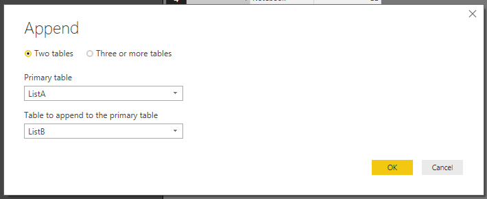
Step 5
In order to append files, you need to select following files as mentioned below. Since in our example, we are using only two tables, multiple tables can be selected if second option “Three or more tables” is clicked. Press “OK” when correct files are selected.
Step 6
You will notice that now both tables are combined and showing collective list.
| 1 | Pencil | 2 |
| 2 | Eraser | 3 |
| 3 | Pen | 5 |
| 4 | Notebook | 11 |
| 1 | Pencil | 2 |
| 2 | Eraser | 3 |
| 5 | Marker | 12 |
| 6 | Whiteboard | 45 |
However this list has duplicate values. These were purposely entered in the list to show you how we can get rid of those.
Step 7
Click on “Remove Rows” icon from the ribbon and select “Remove Duplicates”. This action will give you final list with unique items from both lists.

This will complete your append operation.
Final list will be like below.
| 1 | Pencil | 2 |
| 2 | Eraser | 3 |
| 3 | Pen | 5 |
| 4 | Notebook | 11 |
| 5 | Marker | 12 |
| 6 | Whiteboard | 45 |
Step 8
You can rename new combined table as “Combined_Appended” for this example.
Step 9
Click on “Close and Apply” icon on the ribbon to complete this activity.
Merging Tables
Merging of tables is required when you are combining different tables with some common columns to make use of required columns of other tables. This is helpful in situations where product specification is maintained in one table while product prices are maintained in another. Following tables are used to this scenario.
1- Combined_Appended
2- List C
To import List C table, follow similar steps like mentioned in Step 1 of previous example (Append Tables).
Step 2
Select checkbox of “List C” from the list and click “Edit”
Step 3
You will notice that Power BI Query Editor window will open after previous step.
Note: If for any reason this window is not opening directly, then you have to click on “Edit Query” icon on the ribbon.
Step 4
Right click on Query Pane and select as follows
New Query>Combine>Merge Queries as New

Step 5
Now select files as demonstrated below. After selecting files click on “Code” column in both tables. This will make selected columns gray to identify columns used for merging tables.

Now click on “OK” to confirm merging.
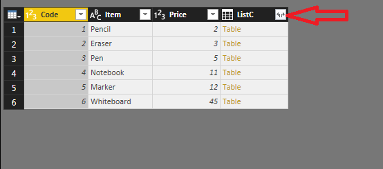
Step 6
Once merged table is loaded, click on the icon on the top right corner as mentioned below to expand table columns.
Step 7
You will see following window like below after completing previous step.

Now select Columns not available in first table to avoid duplicates. I our case we will select only “Box” and “Units” columns. In this example we can deselect “Use original column name as prefix” checkbox.

Click on “OK” to complete this step.
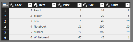
Step 8
You will now see a merged table with combined columns like below.
Step 9
Click on “Close and Apply” icon on the ribbon to complete this activity.
